
THE PROBLEM
Your factory has more capacity than you think
Most business leaders I work with — across diverse range of industries — are convinced they need new machines, more manpower, or a bigger plant before they can grow. They are almost always wrong.
In my experience, I’ve rarely seen a factory operating at its true capacity ceiling. What I do see, repeatedly, is capacity that’s been buried under poor scheduling, invisible queues, batch-size policies, and the silent killer: a single overloaded constraint that the entire system is dancing around without anyone quite realising it.
| “The constraint is not what is working the hardest. It is what is producing the least relative to market demand. Find that, and everything changes.” |
DIAGNOSIS FIRST
How to identify hidden capacity — before you do anything else
Hidden capacity is not a mystery. It leaves signals, and if you know what to look for, you can find it in a single day of focused observation. Here are the eight most reliable indicators I use during an initial diagnostic walk:
| Signal | What to look for | Benchmark / Threshold |
| 01 Queue Asymmetry | Walk the floor — map WIP queue size at each station at 9AM, 12PM, 4PM. Large persistent queues = constraint area. Idle machines downstream = hidden capacity. | Any queue > 4 hours is a signal |
| 02 OEE Below 65% | Measure Availability × Performance × Quality for each machine. Any machine under 65% has significant recoverable capacity without investment. | World class = 85%. Most SMEs: 45–60% |
| 03 Changeover Duration | Time every changeover on critical machines. If setups exceed 90 minutes and operators treat this as normal, you are losing 15–25% capacity on that machine. | > 90 min = immediate SMED candidate |
| 04 Shift Output Gap | Compare day shift vs. night shift output. A gap > 15% is a system design problem, not a people problem. | > 15% gap = policy/system issue |
| 05 First Pass Yield < 90% | Track FPY at each station. Every rejected part consumed capacity producing zero net output. 5% rework = 5% capacity lost. | FPY < 90% = capacity leakage |
| 06 Batch Size Dogma | Ask why batch sizes are what they are. ‘We always did it this way’ is not an engineering answer. | Reduce by 50% and observe flow. Ideally, do SMED before reducing batch size |
| 07 Material Starvation Events | Track how often machines stop due to material, drawing, jig, fixture, or operator absence. Every non-breakdown stop is a policy failure. | Target: zero starvation stops on constraint |
| 08Lead Time / Touch Time Ratio | Measure total lead time vs actual value-adding machine time. Ratio > 10:1 means the part spends 90%+ of its life waiting. | Ratio > 10:1 = major flow problem |
The Hidden Capacity Fingerprint — Typical of mfg. companies
When I run a diagnostic on a first visit, I typically find the following capacity.
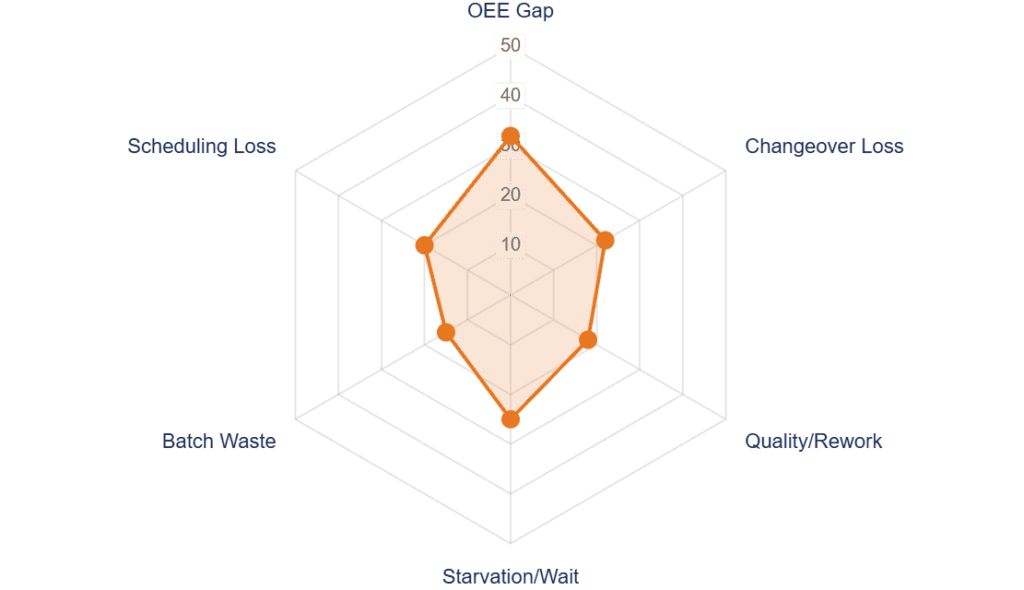
Total recoverable capacity, conservatively: 25–45% of current output — without adding a single machine, person, or rupee of capital.
THE INSIGHT
Finding and exploiting your constraint
Every system has exactly one binding constraint at any given time, and the output of the entire system is determined by that one constraint alone.
| “Improving anything that is not the constraint delivers zero additional throughput (Sales – Truly Variable Cost) . It only creates local efficiency that looks good on a departmental report — while system throughput stays flat.” |
The Focusing approach — Applied to the manufacturing floor
| Step | Action | Shopfloor Translation |
| 1. IDENTIFY | Find the one constraint limiting throughput | Map queues. The process/machine with the biggest, most persistent input queue is usually your constraint. |
| 2. EXPLOIT | Get maximum output from the constraint — no investment | No idle time at constraint. Best operator. No quality holds sitting more than 10 min. Pre-staged materials. |
| 3. SUBORDINATE | Make all other resources serve the constraint’s pace | Release work based on constraint capacity. Cap upstream WIP. Redesign daily meeting around constraint. |
| 4. ELEVATE | Only now consider investment if constraint persists | After steps 2–3, if output is still insufficient, then and only then consider capex to elevate the constraint. |
| 5. REPEAT | Once constraint breaks, find the new one | The constraint moves. Immediately identify where the new bottleneck has formed. |
Drum-Buffer-Rope (DBR) Scheduling — Zero-Cost Flow Control
DBR is the TOC-derived scheduling method that replaces complex MRP-driven release systems. It requires no software, no investment:
- DRUM: The constraint sets the production pace. All other scheduling decisions follow its rhythm.
- BUFFER: A physical WIP buffer (time-based: say 4 hours of work) is placed in front of the constraint. This ensures it never starves.
- ROPE: Work is only released into the system at a rate the constraint can consume. Upstream operations are ‘tied’ to the drum.
The practical result: WIP drops, lead time compresses, and throughput increases — all from a scheduling change that can be implemented with a whiteboard and two meetings.
5 PRACTICAL TACTICS
Increase output without spending a single rupee
Tactic 1: Make the constraint visible — and protect it religiously
Once you identify the constraint machine/process, install a physical WIP buffer in front of it (equivalent to say 4 hours of work). Assign your best operator. Track its utilisation every hour using a simple T-card or whiteboard. A constraint running at 90% vs. 70% utilisation delivers 28% more throughput from the same asset, same shift, same cost base.
Tactic 2: SMED on the constraint — from 3 hours to 80 minutes
Separate internal setup activities (machine must be stopped) from external ones (can be done while machine is running). In most companies, 40–60% of changeover time is external work being done internally — simply because ‘that’s how we do it.’ SMED converts this without buying anything. Every hour saved on the constraint is one additional hour of sellable production per changeover.
Illustration:
| Activity | Before SMED | After SMED | Time Saved |
| Die retrieval and staging | During stop (45 min) | Before stop — external | 45 min |
| Tool pre-heating | During stop (30 min) | Pre-heated in last 30 min of prev run | 30 min |
| First-piece approval wait | 20 min idle post-setup | Inspector pre-positioned | 15 min |
| Documentation / sign-off | 15 min during stop | Prepared in advance | 12 min |
| Total changeover time | 180 minutes | 78 minutes | 102 min (57%) |
Tactic 3: Eliminate productive non-production
Track all the reasons a machine stops other than planned maintenance. These include: waiting for drawing/first-piece approval, tool change, material shortage, operator unavailability, power fluctuations, and quality holds. These are all policy failures. Fixing the top 3 stoppage causes recovers 12–18% OEE within 60 – 90 days — purely through better protocols, signboards, and discipline.
Tactic 4: Reduce batch sizes — counterintuitive but powerful
Cutting batch sizes by half often increases throughput. Smaller batches flow faster, expose problems earlier, and eliminate ‘batch wait’ — the time a part spends waiting for the rest of its batch to complete before moving to the next operation. At one forging plant, halving batch size cut lead time by 38% with zero additional resource or investment.
Tactic 5: Synchronise scheduling to the constraint drum
Do not release work into the system based on raw material availability or sales pressure. Release it based on what the constraint can absorb in the next 4–8 hours. This single change — often implemented with nothing more than a whiteboard and a discipline agreement — prevents upstream pile-ups that mask output capacity and inflate apparent WIP.
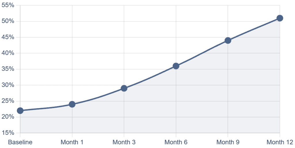
OEE Improvement — Revenue Impact (Illustrative, Rs/ Lakhs/month)
| OEE Level | Units/Month | Revenue @ ₹850/unit (Rs. Lakhs) | Delta vs. 55% OEE |
| 55% (typical SME today) | 2,600 | Rs.22.1 L | Baseline |
| 65% (after discipline improvements) | 3,080 | Rs.26.2 L | +Rs.4.1 L/month |
| 75% (SMED + stoppage elimination) | 3,540 | Rs.30.1 L | +Rs.8.0 L/month |
| 85% (world class) | 4,010 | Rs.34.1 L | +Rs.12.0 L/month |
Note: The variable cost base remains largely fixed. Additional throughput revenue flows directly to gross margin. EBITDA impact is therefore 2–3× the revenue delta shown above.
FLOW & SPEED
Cutting lead time without adding a single resource
Lead time is where customer perception of your competitiveness lives. In B2B manufacturing, a company that can commit to 7-day delivery vs. a competitor’s 21-day wins the order — often at a premium. The paradox: long lead times are almost never a capacity problem. They are a flow problem.
A part spends, on average, less than 10% of its time in value-adding transformation. The rest — 90%+ — is waiting: in queues, for approvals, for setups, for inspection, for transport between departments.
Where lead time actually goes — typical 10-day cycle
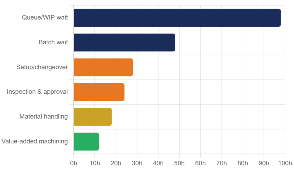
| Category | Hours (of 240 total) | % of Lead Time | Addressable without Capex? |
| Queue / WIP wait at constraint | 98 hours | 41% | Yes — DBR scheduling |
| Batch accumulation wait | 48 hours | 20% | Yes — lot splitting |
| Setup / changeover time | 28 hours | 12% | Yes — SMED |
| Inspection and approval wait | 24 hours | 10% | Yes — inline QC, SPC |
| Material handling / inter-dept move | 18 hours | 7% | Yes — layout / signal redesign |
| Value-added machining time | 12 hours | 5% | N/A — this is production |
| Planned maintenance / breakdowns | 12 hours | 5% | Partially — TPM |
Three lead time contributors to attack immediately
Contributor #1 — Queue length at non-constraints: Limit WIP released into the system using DBR or Kanban signals. Every hour of reduced queue = one hour of reduced lead time. Cap the queue at constraint input to say 3–4 hours.
Contributor #2 — Lot splitting and overlapping operations: Send partial sub-batches to the next operation as they complete, rather than waiting for the full batch. At one auto-component plant, overlapping just two sequential operations cut lead time by 4 days — no investment.
Contributor #3 — Compress inspection and approval cycles: Move inspectors physically closer to the constraint. Implement SPC-based process control to reduce frequency of 100% inspection. These are protocol changes — not capital expenditures.
THE MONEY VIEW
How output and lead time gains translate into ROCE
ROCE (Return on Capital Employed) = EBIT ÷ Capital Employed. For a manufacturer, every rupee of throughput improvement — without adding capital — directly improves ROCE. This is the leverage that makes constraint-based thinking so powerful: you grow the numerator without growing the denominator.
| 2.3×Typical ROCE improvementfrom 25% output gain | Rs.0Additional capital employedin most interventions | 18–26Weeks to ROCE impacton annual P&L | 40–60%EBITDA upliftfrom throughput gain |
ROCE Calculation — Before and After Intervention (Illustrative)
The dramatic ROCE improvement is not magic — it is the consequence of contribution margin leverage. Fixed costs are already being paid. Every additional unit of throughput above the breakeven point flows almost entirely to EBIT.
| Metric | Before Improvement | After Improvement (25% output gain) | Change |
| Monthly Throughput (Rs.Cr ) |
11.4 | 14.25 | 2.85 |
| Total Monthly Costs (Fixed + Variable) | 7.75 | 8.27 | 0.51 |
| Monthly EBIT (Rs. Cr) | 3.65 | 5.99 | 2.34 |
| Annual EBIT (Rs. Cr) | 43.78 | 71.82 | 28.04 |
| Capital Employed (Rs. Cr) | 53 | 53 | No change |
| ROCE (Annual) | 83% | 136% | +53 percentage points |
FROM THE FIELD
Case studies — three transformations, zero capex
| Case 01 — Auto-Component Manufacturer | Tier-2 OEM Supplier [Constraint Identification + DBR] |
SITUATION: A Tier-2 supplier was struggling with 18-day lead times and could not accept additional OEM orders despite a busy shopfloor. Management believed they needed a new CNC machining centre (estimated Rs.2.40 Cr investment).
DIAGNOSIS: Queue mapping revealed that the 4-axis CNC was the system constraint, losing 3.2 hours/shift to setup, first-piece inspection waits, and operator lunch breaks with no alternate coverage. OEE measured at 52% — against a purchased capacity of 95%.
INTERVENTION: Applied SMED on the 4-axis CNC — moved all external setup activities off the machine. Deployed a dedicated setter during shift handovers. Created a 4-hour physical buffer in front of the constraint. Assigned first-piece inspection priority. Scheduled DBR-based work release upstream.
| +34%Output increase | 11 daysLead time (from 18) | Rs.0Capital spent |
Additional monthly throughput generated: Rs.82 lakhs. ROCE improved from 19% to 31% over 8 months. The Rs.2.40 Cr investment was cancelled.
| Case 02 — Plastic Products Manufacturer [Lead Time Compression + Flow Redesign] |
SITUATION: A plastic products manufacturer had a 14-day standard lead time. Three competitors were quoting 7–8 days. The company was losing orders — not on price, but on delivery commitment.
DIAGNOSIS: Touch time per order was only 11 hours across a 14-day cycle. The remaining 229 hours were consumed by batch accumulation (waiting for so called EBQ before releasing to moudling), inter-department transport delays, and a 2 day printing and packaging cycle that included 18 hours of queue wait.
INTERVENTION: Implemented lot splitting — raw material released in sub-batches of 150 instead of 300. Created a visual order-tracking board with daily status. Moved QC inspection inline at moulding rather than end.
| 6 daysLead time (from 14) | +22%Orders won (month 3) | Rs.0Additional investment |
Revenue grew by Rs.22 lakhs/month without adding any machine or person. ROCE improved from 16% to 27% in 9 months.
ACTION PLAN
Your 180-day sprint
Stop planning. Start doing. Here is a 180 day implementation sequence that works regardless of your factory’s size or sector:
| Week | Action | Expected Output |
|---|---|---|
| Week 1–6 | The diagnostic walk: Map WIP queues at 9AM, 12PM, and 4PM for atleast a days. Calculate OEE on top 5 machines primarily low output. List top 3 stoppage reasons per machine. | Queue map, OEE data, stoppage Pareto |
| Week 7–9 | Constraint identification: Analyse queue data. Declare the constraint formally in a team meeting. Assign a constraint champion. | Constraint identified and visible on shopfloor |
| Week 10-18 | Exploit the constraint — 5 quick wins: No idle time at constraint, no quality holds > 10 min, pre-staged materials, SMED workshop (data collection phase), best operator assigned. | 5–12% throughput gain within week 15 |
| Week 19-24 | Subordinate to the constraint: Install 4-hour WIP buffer. Cap work release based on constraint capacity. Redesign daily production meeting around constraint performance. | WIP reduces, flow improves, lead time begins falling |
| Week 24-26 | Measure, celebrate, and iterate: Calculate throughput improvement vs. baseline. Share results with entire team. Update ROCE projection. Identify where the constraint has now moved. | 25–35% throughput improvement visible. Next cycle begins. |
Key metrics to track from Day 1
- Throughput (Rs/day or units/day at the constraint)
- OEE at the constraint machine (%)
- WIP in front of the constraint (hours of buffer)
- Changeover time on the constraint (minutes)
- Lead time by order (days from release to despatch)
- First Pass Yield at constraint (%)
Do not track 10 KPIs. Track these 6. Review them daily at the constraint. The rest of your metrics will follow.
CLOSING THOUGHTS
The factory that grows before its competitors do
Most Indian manufacturers are sitting on 25–45% of untapped throughput capacity. They don’t need more machines, more people, or more capital in first place. They need a new way of seeing their factory — one that asks ‘where is the constraint?’ before asking ‘what shall we buy?’
The companies that will pull ahead in the next 5 years are the ones that master the discipline of doing more with what they already have. Flow-based thinking are not exotic concepts. They are proven engineering frameworks that work in any company & sector.
| “The highest ROCE comes not from investing more, but from extracting more from what you have already invested. That is the philosophy behind every engagement Profound Consulting runs.” |
If you would like to explore what a structured manufacturing floor diagnostic could unlock in your factory, reach out to us at Profound Consulting. In a typical 2-day visit, we identify atleast Rs.1 ~ 3 Cr per month in recoverable throughput for a mid-sized company— and help you build a 180-day roadmap to capture it.
|
PROFOUND CONSULTING Imran Shaikh info@profoundconsulting.in | www.profoundconsulting.in | linkedin.com/in/imranhshaikh-thoughtleader |